Generalized linear models (GLM)

Gist

When an ordinary Linear regression (LM) regression doesn't cut it - maybe your response variable are whole integers or proportions bounded by $[0, 1]$ . Who you gonna call? Generalized linear model (GLM)

Mathematics

For an outcome $Y$ , it is assumed to be generated from a distribution in the Exponential Family. The conditional mean $μ$ depends on the independent variable $X$ . Here:

E (Y | X) = μ = g^{- 1} (X β),

where the expected value of $Y$ conditioned on $X$ is equal to $μ$ which is also equal to the inverse of link function of the linear predictor: $X B$ .

The linear predictor scale is able to range across $(- \infty, \infty)$ , but by applying $g^{- 1}$ to the linear predictors, we are mapping the mean to the appropriate space. For example, if we're interested in just count data (using Poisson distribution), we want the mean to be bound between 0 and infinity.

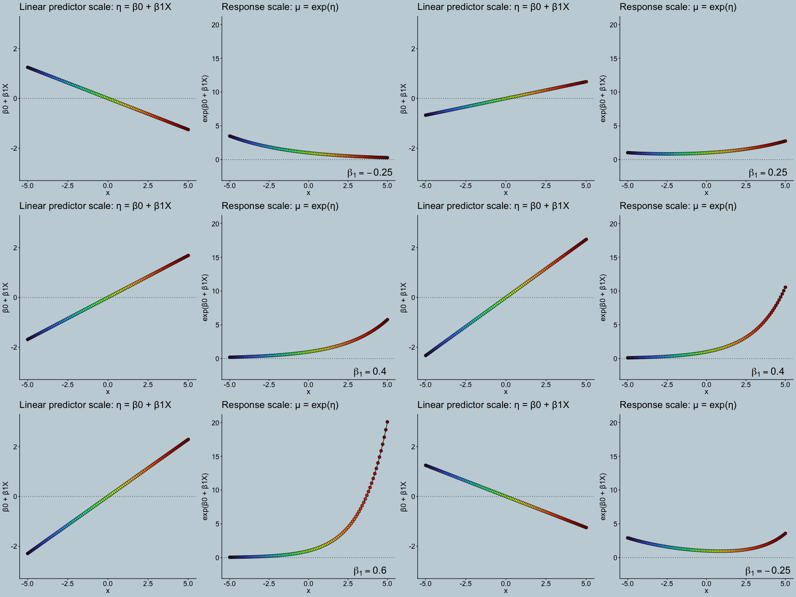
Equivalently, $g (u) = X β$ , meaning that the link function of the mean gets you the linear predictor.

library(dplyr)
library(ggplot2)
library(magick)
library(gganimate)
library(viridis)
library(latex2exp)

response_var <- function(beta0, beta1, time) {
 x   <- seq(-5, 5, by = 0.1)     
 eta <- beta0 + beta1 * x
 mu  <- exp(eta)
 data.frame(x = x, eta = eta, mu = mu, 
            beta0 = beta0,beta1 = beta1,time = time)
}

time1<- response_var(beta0 = 0, beta1 = -0.6, 1)
time1<- response_var(beta0 = 0, beta1 = -0.4, 2)
time2<- response_var(beta0 = 0, beta1 = -0.25, 3)
time3<- response_var(beta0 = 0, beta1 = 0.25, 4)
time1<- response_var(beta0 = 0, beta1 = 0.4, 5)
time4<- response_var(beta0 = 0, beta1 = 0.6, 6)

all_df <- rbind(time1,time2, time3, time4)
label_df <- all_df %>% distinct(time, beta1)

plot_a <- ggplot(all_df, aes(x = x, y = eta, group = 1)) +
 geom_line() +
 geom_point(aes(fill = as.factor(x)), size = 2.5, shape = 21) +
 scale_fill_viridis(discrete = TRUE, option = 'turbo') +
 labs(title = "Linear predictor scale: η = β0 + β1X",  
      y = labs(y = "β0 + β1X"))+
 geom_hline(yintercept = 0, linetype = "dotted") + 
 theme_classic() + 
 theme(legend.position = 'none',
       title = element_text(size = 16),
       plot.background = element_rect(fill = "#C5D3DB", color = "#C5D3DB"),
       panel.background = element_rect(fill = "#C5D3DB", color = "#C5D3DB"),
       panel.grid = element_blank(),
       axis.text = element_text(color = "black", size = 14),
       axis.title = element_text(color = "black", size = 15),
       plot.title = element_text(color = "black"),
       axis.line = element_line(color = "black"),
       legend.background = element_rect(fill = "#C5D3DB"),
 ) + 
 transition_states(time)

a <- animate(plot_a, nframes = 100, fps = 20, width = 400, height = 400)

plot_b <- ggplot(all_df, aes(x = x, y = mu, group =1)) +
 geom_line() +
 geom_point(aes(fill = as.factor(x)), size = 2.5, shape =21) +
 geom_hline(yintercept = 0, linetype = "dotted") + 
 scale_fill_viridis(discrete = TRUE,option = 'turbo') +
 labs(title = "Response scale: μ = exp(η)", 
      y = "exp(β0 + β1X)") +
 geom_text(data = label_df,
           aes(x = 3.9, y = -2,
               label = paste0("beta[1] == ", round(beta1, 2))),
           parse = TRUE, size = 7,color = 'black') +
 theme_classic() + 
 theme(legend.position = 'none',
       title = element_text(size = 16),
       plot.background = element_rect(fill = "#C5D3DB", color = "#C5D3DB"),
       panel.background = element_rect(fill = "#C5D3DB", color = "#C5D3DB"),
       panel.grid = element_blank(),
       axis.text = element_text(color = "black", size = 14),
       axis.title = element_text(color = "black", size = 15),
       plot.title = element_text(color = "black"),
       axis.line = element_line(color = "black"),
       legend.background = element_rect(fill = "#C5D3DB"),
 ) + 
 transition_states(time)



b <- animate(plot_b, nframes = 100, fps = 20, width = 400, height = 400)

a_mgif <- image_read(a)
b_mgif <- image_read(b)

new_gif <- image_append(c(a_mgif[1], b_mgif[1]))
for(i in 2:length(a_mgif)){
 combined <- image_append(c(a_mgif[i], b_mgif[i]))
 new_gif <- c(new_gif, combined)
}

new_gif
anim_save("new_gif.gif", animation = new_gif)

Fitting

Done through Maximum likelihood

Binomial

The link function for Binomial is the logit or probit function.

Normal

The simple Linear regression (LM) is simply a Normal Distribution with an identity function.

Poisson

The link function for Poisson is a natural log.

So $g^{- 1} (X B) = μ$ in this case would be $e x p (X B) = μ$ .
Likewise $g (μ) = X B$ would be $l o g (μ) = X B$ .

glm(Y~X, family = "poisson")

Notes

You can add an offset to account for different "efforts". The offset function tells the function to NOT estimate a coefficient for it.

Interpretation

All of the coefficients should be exponentiated
Given a unit change in 𝑥, the fitted 𝑦̂ changes by $𝑦 (𝑒^{β} - 1)$

GLM the Bayesian way

https://www.y1zhou.com/series/bayesian-stat/bayesian-stat-generalized-linear-models/